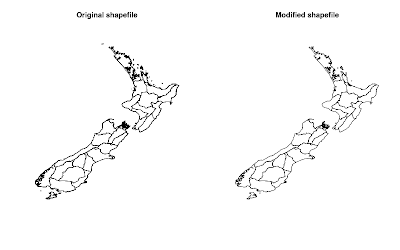
The first thing we needed is to load the packages required and the shapefile itself:
library(maptools)
library(shapefiles)
CCBound <- readShapePoly("nz-area-codes-for-recording-specimen-localities")
CCBound2 <- CCBound
system.time(plot(CCBound2))
user system elapsed
9.537 14.789 142.760
I'm wanting to plot this map multiple times, so waiting 2.5 minutes each time is not at all desirable. The first thing to do was to check out the structure and composition of the object.
str(CCBound, max.level = 3)
sapply(CCBound@polygons, function(x) length(x@Polygons))
62 62 1 1 182 216 2332 81 158 2012 1 22 126 284 45 41 1 35 1 3 1 68 30 78 142 333 1 14 1070 1257 716
area <- lapply(CCBound@polygons, function(x) sapply(x@Polygons, function(y) y@area))
quantile(unlist(area))
0% 25% 50% 75% 100%
3.379739e-10 1.978036e-08 6.223511e-08 2.120671e-07 1.952179
Part of the reason why this is plotting so slowly is the enormous number of polygons to be plotted---9376 in total. We can also see that the majority of these polygons are very small. These polygons represent the myriad of small offshore islands around the NZ coast. As I'm wanting to look at NZ as a whole, these islands are not significant. If we can get rid of these, we will be a long way toward making a leaner, meaner version of the shapefile. We first need to find out what polygons within each larger group are large enough to be worth keeping, then remove them.
mainPolys <- lapply(area, function(x) which(x > 0.001))
CCBound@data <- CCBound@data[-c(1:2),]
CCBound@polygons <- CCBound@polygons[-c(1:2)]
CCBound@plotOrder <- 1:length(CCBound@polygons)
mainPolys <- mainPolys[-c(1:2)]
for(i in 1:length(mainPolys)){
if(length(mainPolys[[i]]) >= 1 && mainPolys[[i]][1] >= 1){
CCBound@polygons[[i]]@Polygons <- CCBound@polygons[[i]]@Polygons[mainPolys[[i]]]
CCBound@polygons[[i]]@plotOrder <- 1:length(CCBound@polygons[[i]]@Polygons)
}
}
When we look at mainPolys, we see the first two larger groupings of polygons have no significantly sized polygons in them. We get rid of these in the following block of data. @plotOrder needs to be the same length as @polygons or else the object will create an error. The second block of code crawls through the object retaining only those polygons we found in mainPolys.
When we plot the returned object:
system.time(plot(CCBound))We see that the plotting time is much more efficient. Depending on our requirements, we could leave it as it is. Being a devil for punishment however, 3 seconds is still a little too slow. There is still a lot of detail in the edges of the main polygons that is unecessary for my requirements. This detail can be simplified using the dp() function in the shapefiles package. Once again, we create a loop that goes through the object simplifying each of the polygons within it. dp() works only on dataframes, so we need to break each @coords matrix into a dataframe, run dp(), then convert it back into a matrix.
user system elapsed
2.536 0.292 3.211
for(i in 1:length(CCBound@polygons)){
for(j in 1:length(CCBound@polygons[[i]]@Polygons)){
temp <- as.data.frame(CCBound@polygons[[i]]@Polygons[[j]]@coords)
names(temp) <- c("x", "y")
temp2 <- dp(temp, 0.01)
CCBound@polygons[[i]]@Polygons[[j]]@coords <- as.matrix(cbind(temp2$x, temp2$y))
}
}
WARNING: This code takes a while to run---around 5 minutes on my machine. The time increases as you decrease the threshold given to dp(). When I had it set to 0.001 it took 7 minutes. However, the time taken to plot the shapefile is now:
system.time(plot(CCBound))Much better! The final thing to do now is to compare the difference between the original and the final product.
user system elapsed
0.072 0.096 0.873
png("comparison.png", width=800, height=500)
layout(matrix(1:2, ncol=2))
plot(CCBound2)
title(main="Original shapefile")
plot(CCBound)
title(main="Modified shapefile")
dev.off()

Looks pretty good to me! When looking at the two of them, you can tell that the modified version has been, well, modified. However, for the purposes I have in mind, the modified version is more than adequate.
Data is of course reproduced with the permission of Landcare Research New Zealand Limited. Get your own copy of it here.
4 comments:
Thanks for your trick. I have been working with raster maps mostly in R and leaving shape files with ArcGIS.
But it is great to know some tricks that R has with shape files.
That is really a good guide for me to manipulating shapefiles in R. Days ago, I just want to the same thing with this blog. I am more familiar with R than ArcGIS. I prefer to do much gis operation in R.
Thanks for sharing such a good experience.
Within the maptools package is a function called "thinnedSpatialPoly" which should simply your code.
library(maptools)
CCBound <- readShapePoly("nz-area-codes-for-recording-specimen-localities.shp")
CCBound2<-thinnedSpatialPoly(CCBound, tolerance=1000, minarea=10000000)
The trick is figuring out what your tolerance and minarea parameters should be. Because this function does take considerable time (much like your own code) I will often take a single polygon from the shapefile to play with until I'm happy with the results. Then I apply those setting to the whole shapefile.
Thanks Sam. That's useful stuff.
Post a Comment