GIS Shapefile of DOC-administered land

The New Zealand Department of Conservation, fondly known as DOC is the department in charge of the bulk of New Zealand's publically owned land. Their best known pieces of real estate are the 14 national parks that conserve some of New Zealand's most iconic landscapes and least modified habitats. Less well known are the legion of scenic reserves and conservation areas that make up a substantial portion of our property. These smaller reserves are no less interesting, and tend to protect small but important areas of near-natural habitat, or intriguing aspects of New Zealand history. Until now, the main way of finding out about them is by stumbling across them while on a road trip, or by word-of-mouth. However, now DOC has released a GIS shapefile that shows the boundaries of all the conservation estate, along with information on what acts of parliament they're protected under and how large the reserve is.

It is important to note that this shapefile only shows those reserves in DOC's ownership and management. Thus, it does not show community-initiated reserves such as Maungatautari Ecological Island or QEII Covenants; nor does it show reserves owned by city councils, like the Auckland Regional Parks or Christchurch's Port Hills Reserves.

Koleopterologische Rundschau

The Austrian entomological journal Koleopterologische Rundschau is an excellent serial that is focussed on beetle taxonomy. It publishes a single issue a year, but this issue is filled to the brim with interesting and informative papers on beetles of all families from Europe and the world. Issues prior to 1990 (Volumes 1-59) are freely available online. PDF versions of papers published since then are also available, but at a cost. Unlike some other outfits though, this cost is actually reasonable; being around 1 Euro per paper.

The Lay of Gudrún (stanzas 100–101)

At the dark doorways
They dinned and hammered;
there was clang of swords
and crash of axes.
The smiths of battle
smote the anvils;
sparked and splintered
spears and helmets.

In they hacked them,
out they hurled them,
bears assailing,
boars defending.
Stones and stairways
streamed and darkened;
day came dimly —
the doors were held.

The Lay of Gudrún, stanzas 100–101.
JRR Tolkien and Christopher Tolkien. (2009). The Legend of Sigurd and Gudrún. Harper Collins.

Changing phylogeny tip labels in R

During the process of molecular systematic research, specimens are given code names and numbers to keep track of data through the pipeline. These can contain a lot of information of relevance to the researcher, but unfortunately are meaningless to others who aren't as involved with the data. On publication, it is necessary to change the names from the code to a label that is more widely understood. This process can be tedious and fiddly, particularly when it needs to be done multiple times.

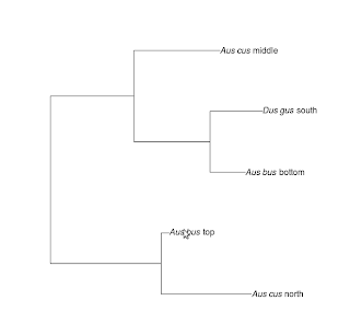
The following is a simple R-based solution for changing the tip labels of phylogenetic trees. First, we need to create a tree and a dataframe containing both the specimen codes and the ultimate labels.

library(ape)
tr <- rtree(5)
d1 <- c("t1","t2","t3","t4","t5")
d2 <- c( "paste(italic('Aus bus'), ' top')", "paste(italic('Aus bus'), ' bottom')", "paste(italic('Aus cus'), ' middle')", "paste(italic('Aus cus'), ' north')", "paste(italic('Dus gus'), ' south')" )
d <- as.data.frame(cbind(label=d1, nlabel=d2))

The code in the nlabel column contains code defining a plottable expression that enables scientific names to be formatted as italics. In my work, I saved this table as a separate file which I call with read.table("file.txt", header=TRUE, sep="\t", stringsAsFactors=FALSE, quote=""). The quote argument is important as it carries the nested quotes through into the dataframe properly.

The business of actually changing the tip labels is done with the following lines:

tr$tip.label<-d[[2]][match(tr$tip.label, d[[1]])]
tr$tip.label<-sapply(tr$tip.label, function(x) parse(text=x))

The first line enters the expressions for the new labels in the correct order. The second line converts the character string into a printable expression.

Plot the tree and voila!

Ubuntu translations

A key part of the Ubuntu philosophy is their emphasis on making computers usable in one's language of choice:

We believe that every computer user should be able to use their software in the language of their choice.

The wiki page provides an entry point for those interested in contributing translations to the project. The process is managed through a project launchpad. Of most interest to me are the Samoan, Maori and Marshallese translations.

Origami

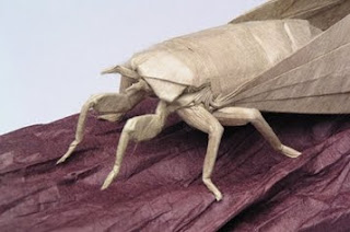
Origami is pretty amazing. While my skills have never progressed beyond the traditional crane, I am always amazed at how people can make a square of paper into something amazing. This website shows a particularly spectacular gallery including the origami cicada pictured above. What's really cool is that it also includes a diagram of the folding patterns for each model. All that's needed is the interpretation of said diagrams, and the time to do it!